Overview
How interested are you this week, do you want to know about linear regression or just how my week was? Hopefully both as I will try to explain how it can be applied and also how I understand it more. I wonder if you will be sad that there will be a gap with my blogs as holidays are next week, if you are going to miss my updates then ask AI to make them instead. If you don’t care enough, then that's fine (and possibly preferred). For me to understand the topic better, actually applying and being able to use it is a huge benefit of learning (and is why this week was interesting).
What was completed
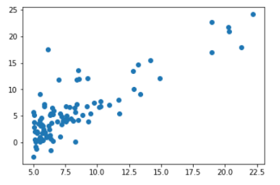
As you should already know the formula for linear regression is: Y = C + BX In this dataset, column zero is the input feature and column 1 is the output variable or dependent variable. We will use column 0 to predict column 1 using the straight-line formula. Currently the code is just displaying the first 4 values. [data (ex1data1.txt)]
import numpy as np
import pandas as pd
df = pd.read_csv('ex1data1.txt', header = None)
print(df.head())
| 0 | 1 | |
|---|---|---|
| 0 | 6.1101 | 17.5920 |
| 1 | 5.5277 | 9.1302 |
| 2 | 8.5186 | 13.6620 |
| 3 | 7.0032 | 11.8540 |
| 4 | 5.8598 | 6.8233 |
Getting the actual values is important but plotting column 1 against column 0 is way more interesting. You can see the trend better and is just better to see and understand. You can see how there is more data in the bottom left, but more importantly the upward straight line that you can see (by imagining)
The code below is basically working to make the line of best fit and then actually graphing it. It does many calculations using the data (data itself and length of data), which all are working so that it can predict a Y value given an X. The predictions will only be across a solid line, and as such not as accurate as some ML algorithms can achieve.
# Initialize the theta values
theta = [0,0]
# Define the hypothesis and the cost function (using the formula)
def hypothesis(theta, X):
return theta[0] + theta[1]*X
def cost_calc(theta, X, y):
return (1/2*m) * np.sum((hypothesis(theta, X) - y)**2)
# Calculate the number of training data as the length of the DataFrame and define the function for gradient descent
m = len(df)
def gradient_descent(theta, X, y, epoch, alpha):
cost = []
i = 0
while i < epoch:
hx = hypothesis(theta, X)
theta[0] -= alpha*(sum(hx-y)/m)
theta[1] -= (alpha * np.sum((hx - y) * X))/m
cost.append(cost_calc(theta, X, y))
i += 1
return theta, cost
# Predicting function
def predict(theta, X, y, epoch, alpha):
theta, cost = gradient_descent(theta, X, y, epoch, alpha)
return hypothesis(theta, X), cost, theta
# Use the predict function to preduct the value
y_predict, cost, theta = predict(theta, df[0], df[1], 2000, 0.01)
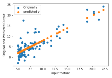
# Now plot the original y and the hypothesis or the predicted y in the same graph.
import matplotlib.pyplot as plt
plt.figure()
plt.scatter(df[0], df[1], label = 'Original y')
plt.scatter(df[0], y_predict, label = 'predicted y')
plt.legend(loc = "upper left")
plt.xlabel("input feature")
plt.ylabel("Original and Predicted Output")
plt.show()
As you can see, the predicted values (using the X axis) make a straight linier line which is somewhat accurate. It would be closer is the data didn’t vary as much, but as an initial prediction it is fairly good. Later on, I can predict the input feature of 100 or something else and assuming the data is still linear, I can guess pretty actually the Y value.
Remember that we wanted to keep track of the cost function in each iteration. To do this we can plot the cost function on a scatter graph. Our purpose was to optimize the theta values to minimize the cost. This graph shows that the cost went down drastically in the beginning and then it became stable. That means the theta values are optimized correctly as we expected.
plt.figure()
plt.scatter(range(0, len(cost)), cost)
plt.show()
Reflection
How applicable is this to data science?
Linear regression is very applicable to data science (analysing data). It is a useful tool for finding the trend and then using it to predict the future. I can very simply ask for some data and only have to supply half the information I will get back (but I still need to give all the data first). The line of best fit has been mentioned many times my me, this is because it shows the trend. Another reason this is data science related, is that I am learning about it in the data science course.
How did you help others?
Occasionally, I have tried to help others. Sometimes it is as basic as helping the to understand a part of a task (in my understanding) or it is to just talk about it to my classmates. This task specifically I did ask some questions (so they helped me!), and this was very helpful and makes me want to continue to help them to be better. In some ways you could expect me to not want to help as then I have better competition, it works both ways and it is fun to explain your thoughts.
Exited for next term?
I am very excited for the holidays, the extra sleeping, with less stress of school. I still have some assignments due very soon after term starts again so still some things to do, but I am looking forward to my next assignment that will be a major project. This excitement may be short lived, and I may want holidays again. However, a future job doesn’t work that way, and I need to continue to think of the positives of each thing (including assignments).